For the purpose of this post, reproducibility means that running the same code on the same input should always yield the exact same result.

Imagine a data scientist who is running a linear regression model. There are situations where it is normal to expect regression coefficients that can vary each time the same model is run on the same input, e.g. if the underlying algorithm uses the stochastic gradient descent method. The reason is there is already some randomness in the underlying algorithm. But if we know that the algorithm does not involve any randomness, is it possible that we can get different regression coefficients from different runs?

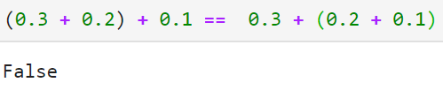
Let’s suppose we would like to solve a system of linear equations \(Ax=b\). Note that a large number of numerical algorithms used in machine learning and statistics require solving such systems and that includes the linear regression model. We will solve the \(Ax=b\) system using Python NumPy function numpy.linalg.solve. The matrix A is a square matrix of size 13 and b is a vector of all zeros except the last element. That last element will be calculated in two ways; first as (0.3 + 0.2) + 0.1, then as 0.3 + (0.2 + 0.1). Of course, the addition is associative, so mathematically both operations give the same number 0.6. The following Python snippet does that:

import numpy as np

n = 13

# create a square matrix of size 13
A = np.empty([n, n], dtype='float')
for i in range(0, n):
    for j in range(0, n):
        A[i, j] = 1.0 / float((i + j + 1))

# create two b vectors where the last entry is calculated from function1 and function2.
b1 = np.zeros(n)
b2 = np.zeros(n)

def function1(array):
    return (array[0] + array[1]) + array[2]

def function2(array):
    return array[0] + (array[1] + array[2])

num_array = [0.3, 0.2, 0.1]

# mathematically b1=b2
b1[n - 1] = function1(num_array)
b2[n - 1] = function2(num_array)

Finally, solve the equations \(Ax=b1\) and \(Ax=b2\).

x1 = np.linalg.solve(A, b1)
x2 = np.linalg.solve(A, b2)

diff = x1 - x2
print(diff)
[  0.0753746   -0.58719635   3.66786194  -9.62109375  10.94921875
  -1.640625   -10.9375      13.875       -7.           0.5
   1.          -0.5          0.0859375 ]

Note that the difference between the coefficients x1[7] and x2[7] is larger than 13! Does the numpy.linalg.solve method have any randomness in it? When we look at the NumPy documentation, we see that it uses the LAPACK method gesv, and that algorithm does not have any randomness in it.

The only reasonable cause of this difference could be in b1 and b2. Indeed when we check the value, we see b2[12] - b1[12]= 1.1102230246251565e-16

So here we have an example of a calculation in floating-point computer arithmetic where the usual associativity of addition is not satisfied exactly! There is, in fact, a whole field of numerical analysis which studies the estimation and control of round-off errors arising from the use of floating-point arithmetic such as this one.

The second surprising observation here is that a difference in two numbers as small as the order of 1e-16 could lead to such different results when it comes to solving \(Ax=b\). Note that I have chosen the matrix A that way for a reason: It is known as the Hilbert matrix which has a huge condition number. In other words, our problem is ill-conditioned meaning that a small perturbation in the input can generate a large difference in the output. Of course, not all systems are ill-conditioned, and many times a small difference in the input would not lead to such a big difference. But imagine a data science production pipeline that runs such computations thousands of times, eventually, an ill-conditioned system might be encountered. For more information on the subject, a very good reference for numerical algorithms is Higham’s book [1].

The reader might argue that this example does not provide exactly the same input since we calculated two different right-hand side b’s with a tiny difference. However, it is extremely difficult to avoid situations like this in practice. Note that b itself typically would be the result of a computation pipeline and we might not have control over the order in which a summation is performed. A common case would be the MapReduce paradigm in Hadoop or Spark calculating a simple aggregated sum. Then two different runs of the same code on the same input can generate different orders in which the sums are evaluated, one such as (0.3 + 0.2) + 0.1, and another as 0.3 + (0.2 + 0.1). And once that has happened, depending on the nature of the subsequent operations, one can get dramatically different results as above!

Perhaps more surprising is the fact that this behavior is not specific to the MapReduce paradigm. For example, the Intel website [2] clearly states when talking about reproducability that …“Many software tools don’t provide exactly reproducible results by default” and that “…reproducibility comes at some cost in performance.” This is the case when exactly the same processor is used for multiple runs of the same code on the same input.

When different processors with different architectures are used, the situation seems even worse [2]: “ Likewise, there’s no way to ensure reproducibility between builds using the Intel Compiler and builds using compilers from other vendors.”

Now that we have seen it is very hard to avoid getting occasionally different results in floating-point arithmetic, however small the difference can be, the next question is can we avoid ill-conditioned systems? If so, the subsequent operations would not propagate the resulting errors in the previous steps and reproducability would be easier to maintain. The answer is that it depends on the application. A well-known case is again our motivating example of linear regression in statistics. It is common to have various degrees of multicollinearity in linear regression which leads to ill-conditioned systems, and that can be alleviated with the addition of a regularization term. Another common way in the regression setting is to identify the multicollinearity and remove certain variables from the model.

Another scenario where ill-conditioned matrices appear might be in an optimization algorithm. Note that this is even more subtle because we typically don’t have much control over how the inner calculations of optimization software are performed. If the underlying algorithm does not take special precautions (as is typically the case in open-source software), the optimal solution would be extremely sensitive to the perturbations in the input data. In that case, the modeler would have to perform some sensitivity analysis and identify whether ill-conditioned systems might appear during the execution of the algorithm.

The common saying that “there is no such thing as a free lunch” applies well when it comes to finite-precision computation.

[1] N. J. Higham. Accuracy and Stability of Numerical Algorithms. Second edition. Society for Industrial and Applied Mathematics, 2002.

[2] https://techdecoded.intel.io/resources/floating-point-reproducibility-in-intel-software-tools/#gs.6ob68t